Running a coordinated release across multiple repos, tagging in the right order and making sure nothing goes out before its dependency, is easy to get wrong when you are doing it manually every time.

I built Shipit around the same plan/apply idea as Terraform. Before anything is pushed you see exactly what will happen: which commits are included, what the tag name will be, what the PR description will say. You review it, then apply it.

A config file defines your projects and their pipelines. Each step is either a branch-to-branch merge (b2b) or a branch-to-tag release (b2t):

projects:
  - name: api-common
    pipeline:
      - type: b2b
        source: dev
        target: main
      - type: b2t
        source: main
  - name: api-service
    pipeline:
      - type: b2b
        source: dev
        target: main
      - type: b2t
        source: main
  - name: frontend
    pipeline:
      - type: b2b
        source: dev
        target: main
      - type: b2t
        source: main

My team uses this for our weekly releases. The plan files also serve as a historical record of every release, including what shipped, when, and what changed.

gitshipit.net

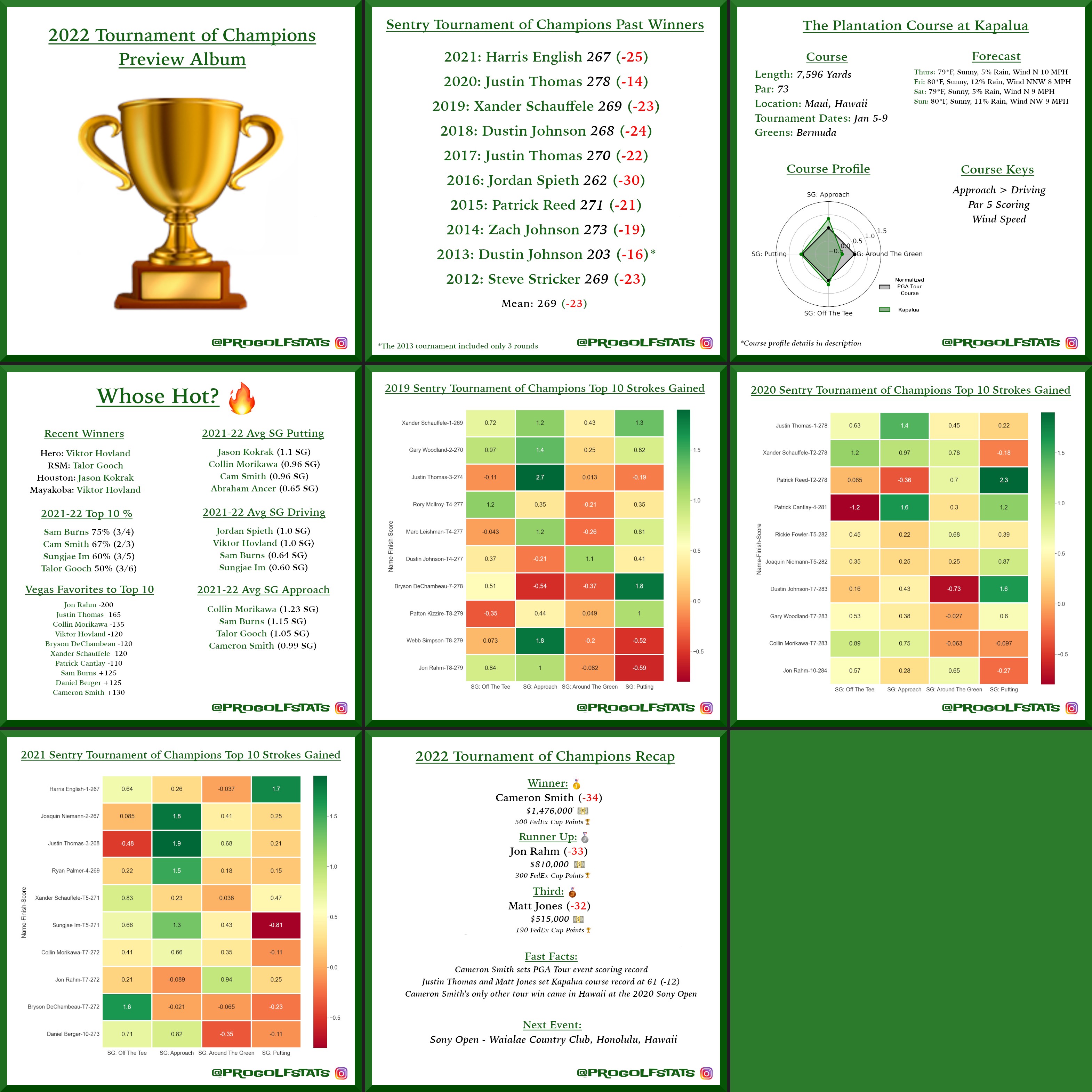
Here is a look at a strokes gained breakdown, past winners, course overviews and more for the first five tournaments of the season. The data is collected from pgatour.com through a pipeline I built that stores the results as Parquet files on AWS S3. Click or tap an image to zoom in.

Sentry Tournament of Champions

‹

›

×

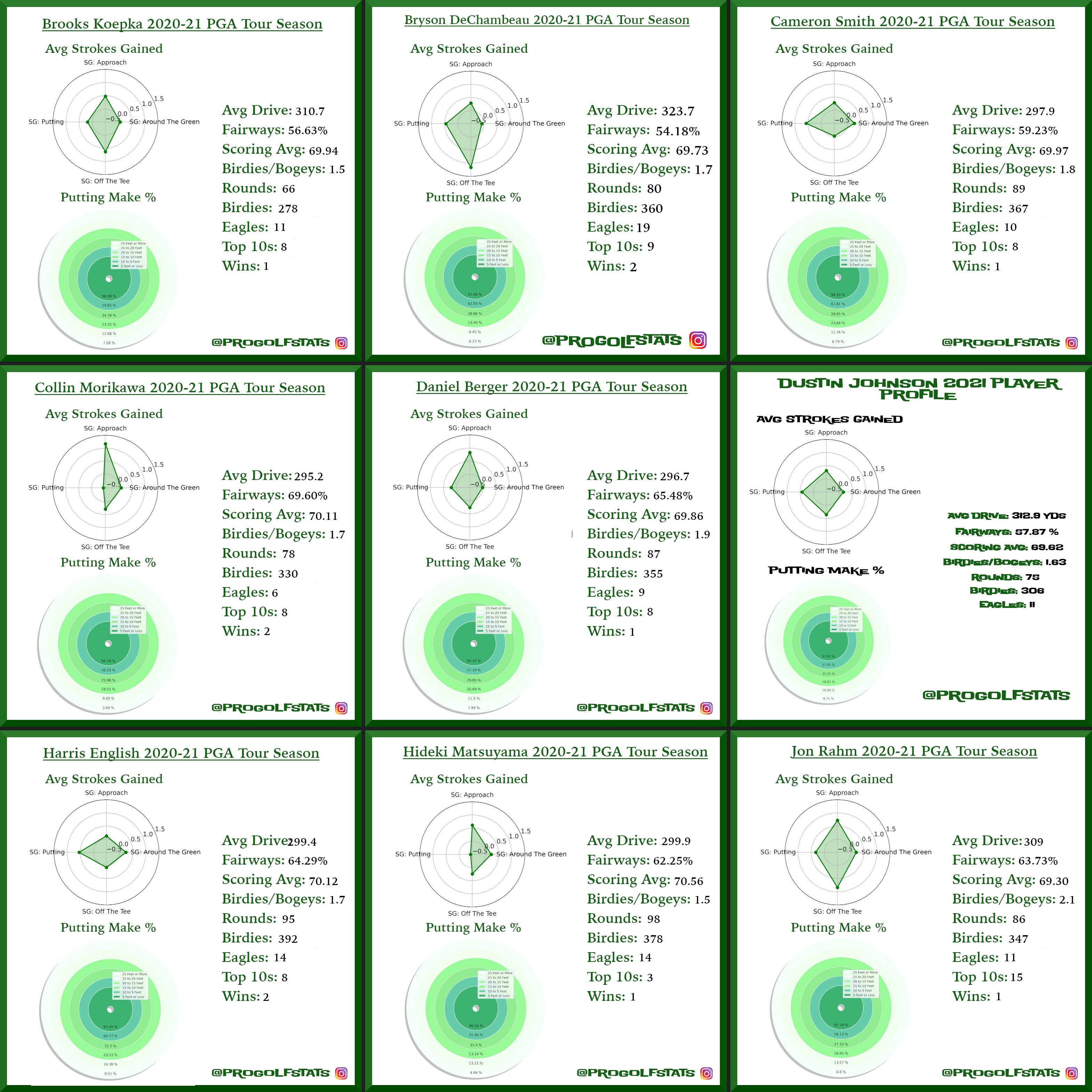
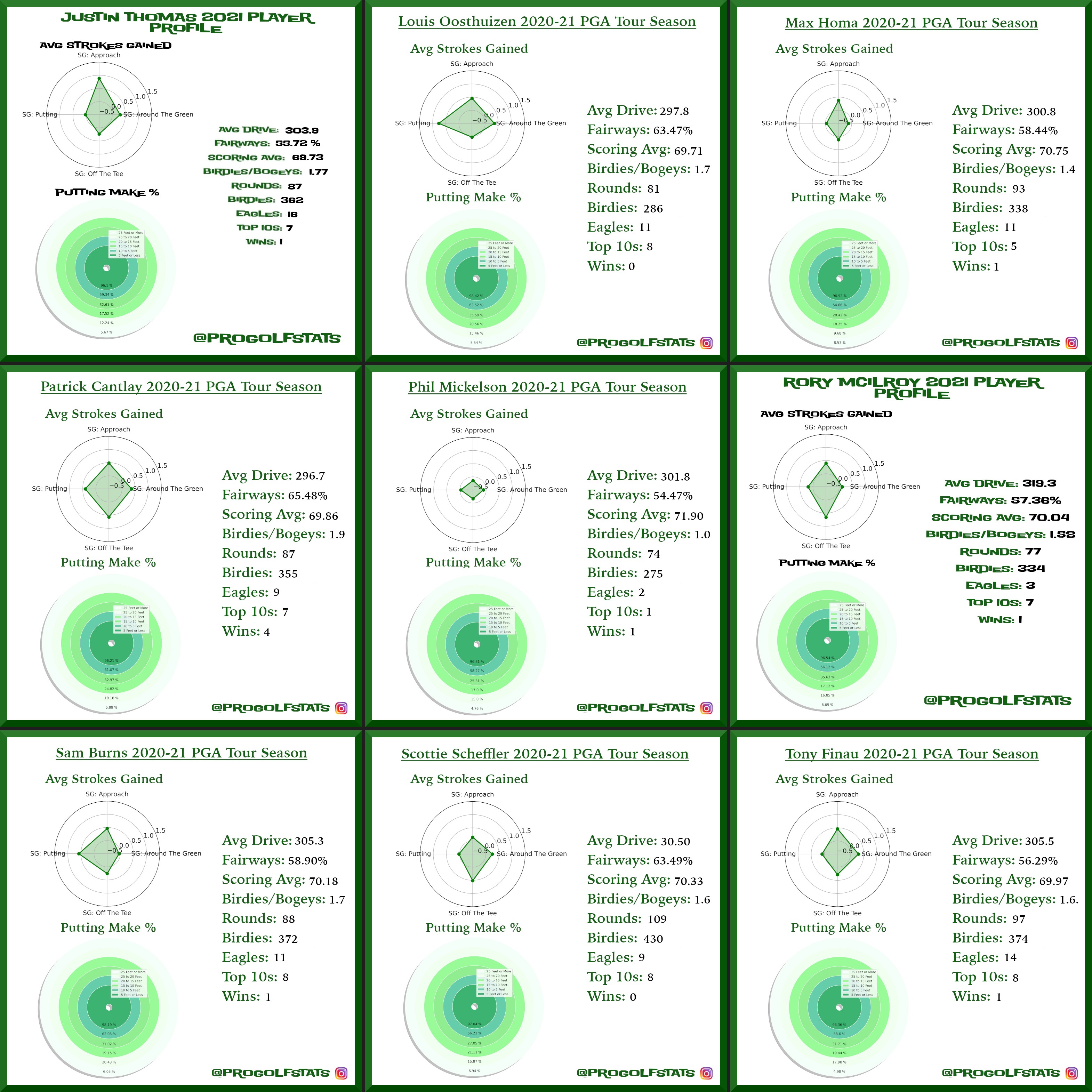
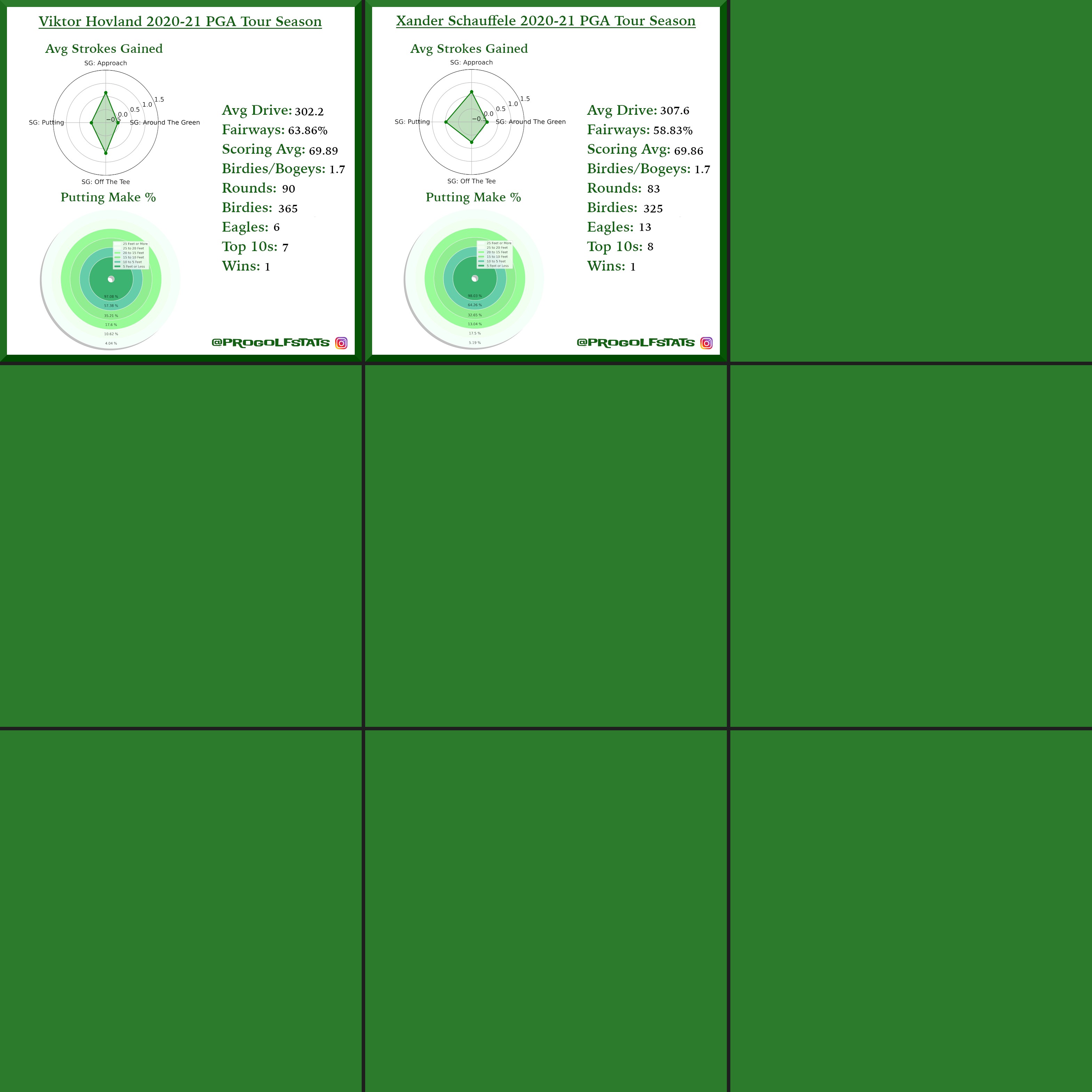
A look at strokes gained profiles for the top players on the 2021 PGA Tour. The data behind these visuals is gathered from pgatour.com through a pipeline I built that collects and stores the results as Parquet files on AWS S3. Click or tap an image to zoom in.

1 of 3

‹

›

×

I completed the Accelerated Computer Science Fundamentals specialization on Coursera, a three-course sequence offered by the University of Illinois Urbana-Champaign.

The specialization covers the foundations of computer science through three courses:

• Object-Oriented Data Structures in C++
• Ordered Data Structures
• Unordered Data Structures

Topics include basic object-oriented programming, asymptotic algorithmic runtime analysis, and the implementation of core data structures: arrays, hash tables, linked lists, trees, heaps, and graphs. Algorithms for traversals, rebalancing, and shortest paths round out the curriculum.

I created and released djangorestframework-mvt through Corteva’s official open source GitHub. It is an extension for Django REST Framework that creates views which serialize model data into Google Protobuf encoded Mapbox Vector Tiles via PostgreSQL and PostGIS.

The package makes it straightforward to serve dynamic vector tiles directly from a PostGIS database without an intermediate tile server. Install it with pip install djangorestframework-mvt and point a DRF view at a model with a geometry field.

It is officially listed on awesome-vector-tiles, a curated list of vector tile tools and servers maintained by Mapbox.

For a full breakdown of the approach behind serving dynamic vector tiles from PostGIS, see the Crunchy Data write-up.

I released Elizur, an open source Python package for actuaries, finance professionals, and students. It is named in honor of Elizur Wright, a 19th century mathematician known as the father of life insurance.

The package helps with calculating annuity present and future values and cash flow expected present values. It accepts both single values and NumPy arrays for vectorized operations and only requires NumPy at runtime.

import elizur.life.annuity as ann

ann.annuity_pv(n=10, i=0.07)
# 7.023581540932602

ann.annuity_pv(n=[10, 20], i=[0.07, 0.08])
# array([7.02358154, 9.81814741])

from elizur.life import expected_present_value

expected_present_value(
    cash_flows=(10, 11, 12),
    probabilities=(0.99, 0.98, 0.97),
    interest_rates=(0.05, 0.06, 0.07)
)
# 28.88814436019514

Install it with pip install elizur. The source and documentation are on GitHub.

At Pioneer I have been building an API that paginates through thousands of land parcel sales records. Under load the responses were slower than expected, so I dug into the flask-sqlalchemy pagination internals.

The issue is that every call to .paginate() runs a full COUNT(*) against the table to calculate the total number of pages. On a large table that count is expensive, and it runs on every single request regardless of whether the caller needs that information.

I opened a pull request to make the count optional. The fix adds a count parameter to .paginate() that defaults to True for backwards compatibility but lets you opt out when you do not need the total page count.

# before, always counts the full table
page = query.paginate(page=2, per_page=25)

# after, skip the COUNT(*) when you don't need it
page = query.paginate(page=2, per_page=25, count=False)

It is a small change, but it meaningfully reduces response times for any endpoint paginating through a large dataset without needing to report back a total page count.

A few days ago a coworker asked why Python returned different values for the example below:

(~)$ python
>>> 4.32 - 3.92
0.40000000000000036
>>> 3.32 - 2.92
0.3999999999999999

As you can see both of these differences would be 0.40 in base 10, but why aren’t they in Python?

The short answer: four in binary is 100 and three is 11, so four takes one more bit to represent. Floating point numbers have a fixed bit budget, so the fractional parts of 4.32 and 3.32 end up stored differently.

The rest of this post walks through the details. I used a decimal-to-IEEE-754 converter and a binary-to-decimal converter along the way to keep things readable.

That bit budget is finite by design. Irrational numbers can never be represented exactly, and rational numbers with long fractional parts may not fit either. Something has to give, and IEEE 754 is the standard that defines how.

The IEEE 754 specifies a standard for floating-point computation. It defines formats, rounding rules, operations, and exception handling. The standard storage format for double-precision floating-points includes 1 bit for the sign of the number, 11 bits for the exponent, and 52 bits for the mantissa. The value of an IEEE 754 double-precision floating point is computed as: -1 ^ sign * mantissa * 2 ^ exponent. When a number is represented this way it is in scientific notation.

Whew. After you’ve digested all of the above we can finally address why the example above returns two different results for sets of numbers equidistant apart.

#       s exponent           mantissa
4.32: 0 10000000001 0001010001111010111000010100011110101110000101001000
3.32: 0 10000000000 1010100011110101110000101000111101011100001010001111

#       binary
4.32: 100.010100011110101110000101000111101011100001010 [01000]
3.32:  11.0101000111101011100001010001111010111000010100 [01111]

At a quick glance you can see that the fractional portion of 4.32 and 3.32 in binary follow the same pattern until their last five bits. Due to the IEEE 754 formatting restrictions, 4.32 must use one less bit to represent 0.32 than 3.32. This is because the mantissa is only allowed 52 bits and 4 (100 in binary) takes up one more bit than 3 (11 in binary). Even though we entered 0.32 for the fractional portion of 4.32 and 3.32 in the interpreter, Python can’t store their values exactly the same. Below is a translation of 4.32 and 3.32’s bracketed binary fractional values to decimal.

4.32's bracketed fractional value in binary
0.000000000000000000000000000000000000000000000 [01000]

4.32's bracketed fractional value converted to decimal
0.00000000000000710542735760100185871124267578125

3.32's bracketed fractional value in binary
0.0000000000000000000000000000000000000000000000 [01111]

3.32's bracketed fractional value converted to decimal
0.000000000000006661338147750939242541790008544921875

error between the two bracketed fractional values in decimal
4.440892098500626e-16

Below we revisit our initial example and compare the error between the two representations of 0.4.

(~)$ python
>>> x = 4.32 - 3.92
>>> x
0.40000000000000036
>>> y = 3.32 - 2.92
>>> y
0.3999999999999999
>>> x - y # error between the two terms
4.440892098500626e-16

You can now see the error due to bit shaving and the error between the two values presented to us by Python are the same!